Life Data Analysis Part IV - Mixture Models

Segmented Regression and EM Algorithm

Tim-Gunnar Hensel

David Barkemeyer

2022-03-30

In this vignette two methods for the separation of mixture models are presented. A mixture model can be assumed, if the points in a probability plot show one or more changes in slope, depict one or several saddle points or follow an S-shape. A mixed distribution often represents the combination of multiple failure modes and thus must be split in its components to get reasonable results in further analyses.

Segmented regression aims to detect breakpoints in the sample data from which a split in subgroups can be made. The expectation-maximization (EM) algorithm is a computation-intensive method that iteratively tries to maximize a likelihood function, which is weighted by posterior probabilities. These are conditional probabilities that an observation belongs to subgroup k.

In the following, the focus is on the application of these methods and their visualizations using the functions mixmod_regression(), mixmod_em(), plot_prob() and plot_mod().

Data: Voltage Stress Test

To apply the introduced methods the dataset voltage is used. The dataset contains observations for units that were passed to a high voltage stress test. hours indicates the number of hours until a failure occurs or the number of hours until a unit was taken out of the test and has not failed. status is a flag variable and describes the condition of a unit. If a unit has failed the flag is 1 and 0 otherwise. The dataset is taken from Reliability Analysis by Failure Mode ¹.

For consistent handling of the data, {weibulltools} introduces the function reliability_data() that converts the original dataset into a wt_reliability_data object. This formatted object allows to easily apply the presented methods.

voltage_tbl <- reliability_data(data = voltage, x = hours, status = status)
voltage_tbl
#> Reliability Data with characteristic x: 'hours':
#> # A tibble: 58 x 3
#>        x status id   
#>    <dbl>  <dbl> <chr>
#>  1     2      1 ID1  
#>  2    28      1 ID2  
#>  3    67      0 ID3  
#>  4   119      1 ID4  
#>  5   179      0 ID5  
#>  6   236      1 ID6  
#>  7   282      1 ID7  
#>  8   317      1 ID8  
#>  9   348      1 ID9  
#> 10   387      1 ID10 
#> # ... with 48 more rows

Probability Plot for Voltage Stress Test Data

To get an intuition whether one can assume the presence of a mixture model, a Weibull probability plot is constructed.

# Estimating failure probabilities: 
voltage_cdf <- estimate_cdf(voltage_tbl, "johnson")

# Probability plot: 
weibull_plot <- plot_prob(
  voltage_cdf,
  distribution = "weibull", 
  title_main = "Weibull Probability Plot", 
  title_x = "Time in Hours", 
  title_y = "Probability of Failure in %",
  title_trace = "Defectives",
  plot_method = "ggplot2"
)

weibull_plot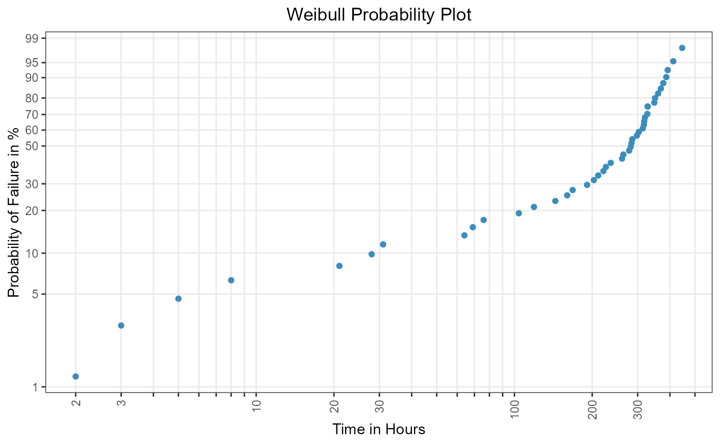

Figure 1: Plotting positions in Weibull grid.

Since there is one obvious slope change in the Weibull probability plot of Figure 1, the appearance of a mixture model consisting of two subgroups is strengthened.

Segmented Regression with {weibulltools}

The method of segmented regression is implemented in the function mixmod_regression(). If a breakpoint was detected, the failure data is separated by that point. After breakpoint detection the function rank_regression() is called inside mixmod_regression() and is used to estimate the distribution parameters of the subgroups. The visualization of the obtained results is done by functions plot_prob() and plot_mod().

# Applying mixmod_regression(): 
mixreg_weib <- mixmod_regression(
  x = voltage_cdf, 
  distribution = "weibull", 
  k = 2
)

mixreg_weib
#> Mixmod Regression:
#> Subgroup 1:
#>    Rank Regression 
#>     Coefficients: 
#>        mu  sigma   
#>     6.910  1.566   
#>  
#> Subgroup 2:
#>    Rank Regression 
#>     Coefficients: 
#>         mu   sigma   
#>     5.7141  0.3048   
#> 

# Using plot_prob_mix(). 
mix_reg_plot <- plot_prob(
  x = mixreg_weib, 
  title_main = "Weibull Mixture Regression", 
  title_x = "Time in Hours", 
  title_y = "Probability of Failure", 
  title_trace = "Subgroup",
  plot_method = "ggplot2"
)

mix_reg_plot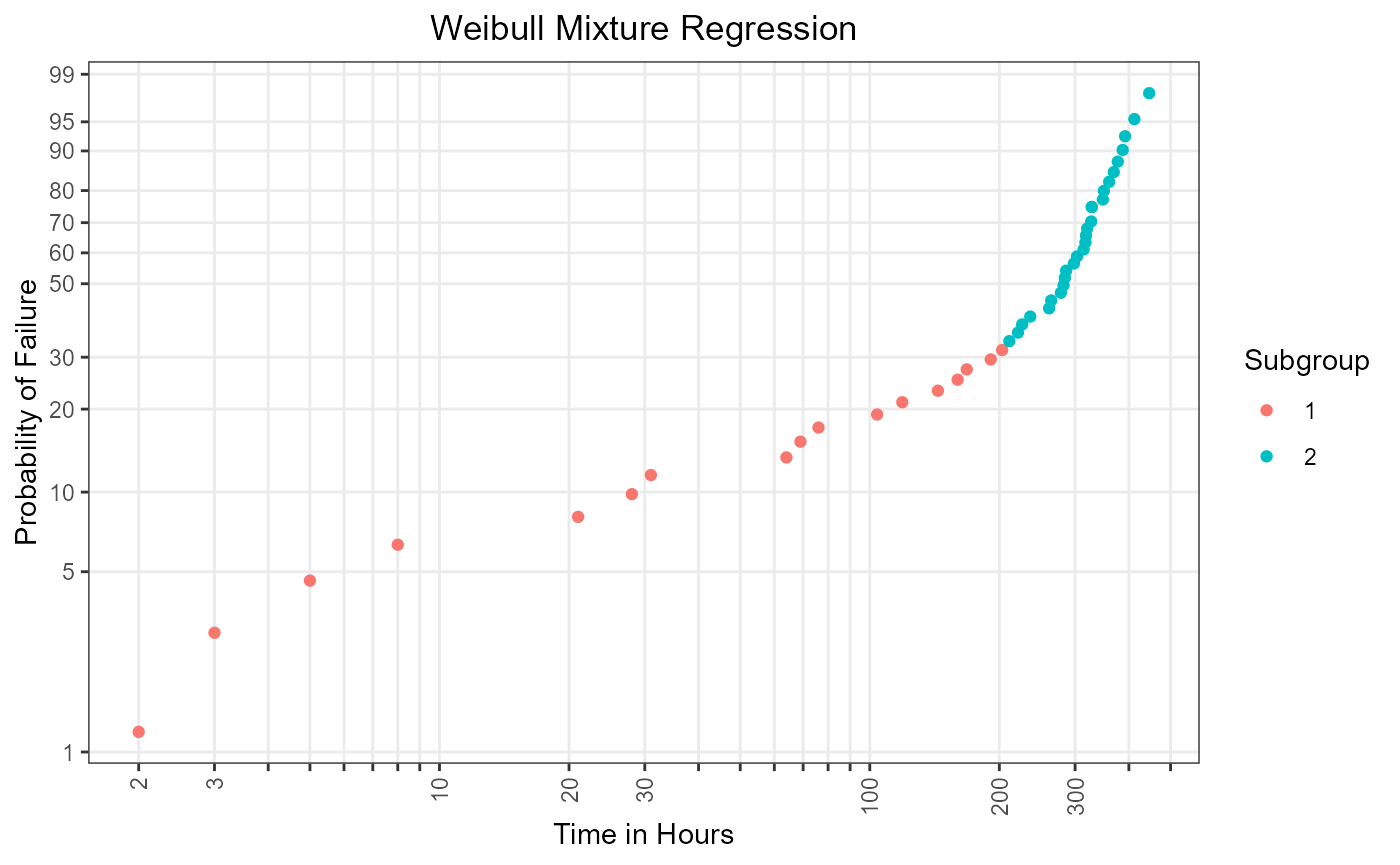

Figure 2: Subgroup-specific plotting positions using segmented regression.

# Using plot_mod() to visualize regression lines of subgroups: 
mix_reg_lines <- plot_mod(
  mix_reg_plot, 
  x = mixreg_weib, 
  title_trace = "Fitted Line"
)

mix_reg_lines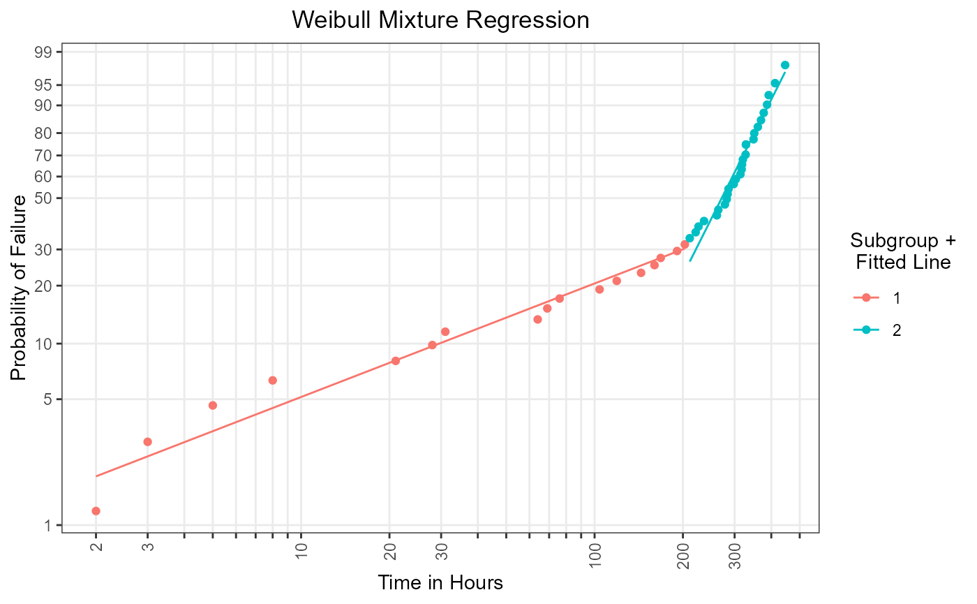

Figure 3: Subgroup-specific regression lines using segmented regression.

The method has separated the data into \(k = 2\) subgroups. This can bee seen in Figure 2 and Figure 3. An upside of this function is that the segmentation is done in a comprehensible manner.

Furthermore, the segmentation process can be done automatically by setting k = NULL. The danger here, however, is an overestimation of the breakpoints.

To sum up, this function should give an intention of the existence of a mixture model. An in-depth analysis should be done afterwards.

EM Algorithm with {weibulltools}

The EM algorithm can be applied through the usage of the function mixmod_em(). In contrast to mixmod_regression(), this method does not support an automatic separation routine and therefore k, the number of subgroups, must always be specified.

The obtained results can be also visualized by the functions plot_prob() and plot_mod().

# Applying mixmod_regression(): 
mix_em_weib <- mixmod_em(
  x = voltage_tbl, 
  distribution = "weibull",
  k = 2
)

mix_em_weib
#> Mixmod EM:
#> Subgroup 1:
#>    Maximum Likelihood Estimation 
#>     Coefficients: 
#>        mu  sigma   
#>     4.244  1.214   
#>  
#> Subgroup 2:
#>    Maximum Likelihood Estimation 
#>     Coefficients: 
#>         mu   sigma   
#>     5.8001  0.2081   
#>  
#> EM Results:
#>    A priori 
#>     0.2574081 0.7425919 
#> 

# Using plot_prob(): 
mix_em_plot <- plot_prob(
  x = mix_em_weib,
  title_main = "Weibull Mixture EM", 
  title_x = "Time in Hours", 
  title_y = "Probability of Failure", 
  title_trace = "Subgroup",
  plot_method = "ggplot2"
)

mix_em_plot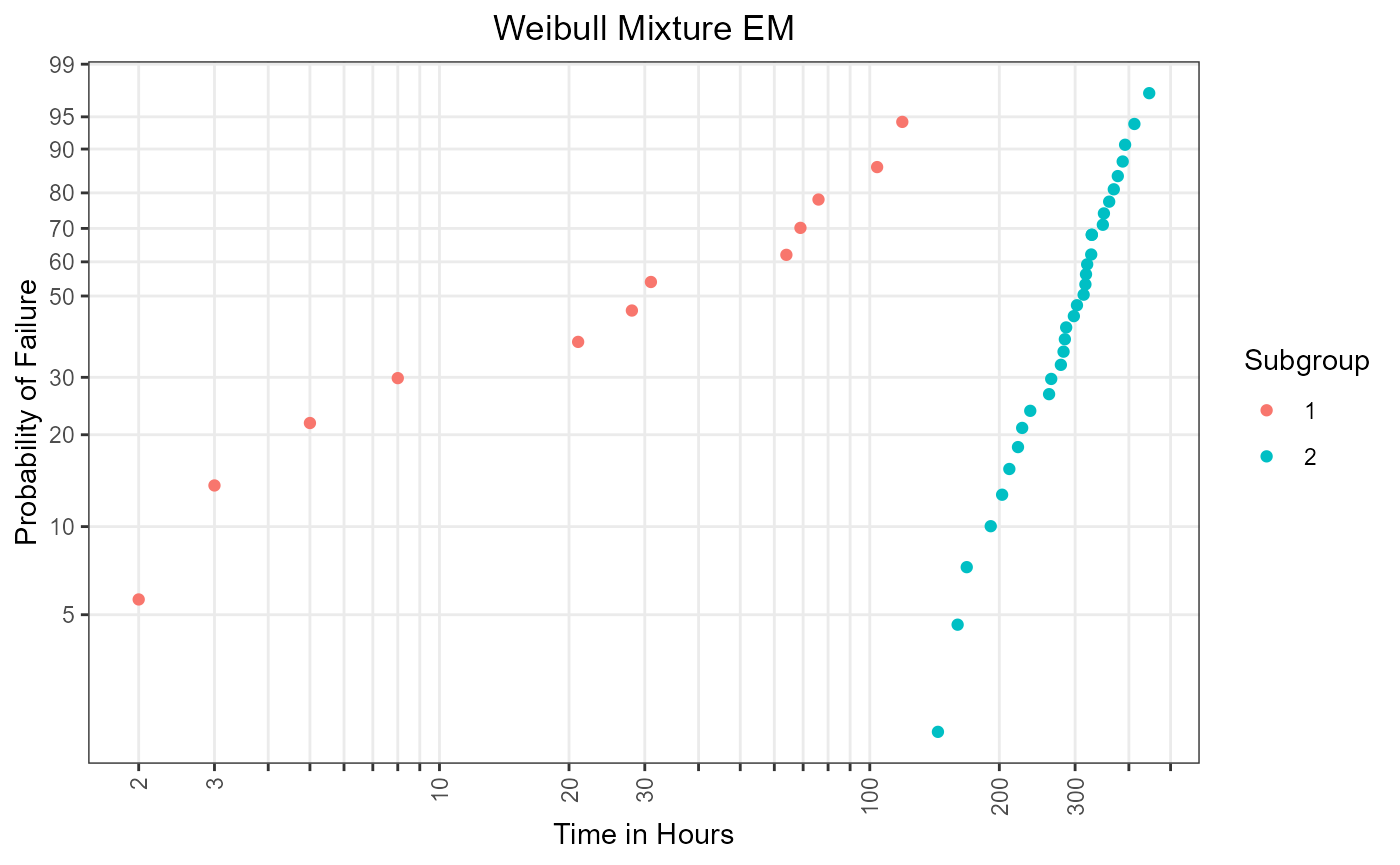

Figure 4: Subgroup-specific plotting positions using EM algorithm.

# Using plot_mod() to visualize regression lines of subgroups: 
mix_em_lines <- plot_mod(
  mix_em_plot, 
  x = mix_em_weib, 
  title_trace = "Fitted Line"
)

mix_em_lines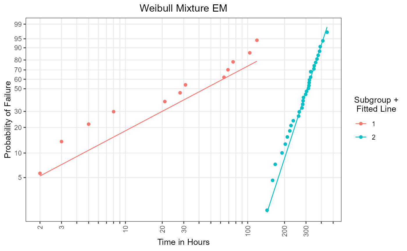

Figure 5: Subgroup-specific regression lines using EM algorithm.

One advantage over mixmod_regression() is, that the EM algorithm can also assign censored items to a specific subgroup. Hence, an individual analysis of the mixing components, depicted in Figure 4 and Figure 5, is possible. In conclusion an analysis of a mixture model using mixmod_em() is statistically founded.

---

1. Doganaksoy, N.; Hahn, G.; Meeker, W. Q.: Reliability Analysis by Failure Mode, Quality Progress, 35(6), 47-52, 2002↩︎