Life Data Analysis Part II - Estimation Methods for Parametric Lifetime Models
Rank Regression and Maximum Likelihood
Tim-Gunnar Hensel
David Barkemeyer
2022-03-30
Source:vignettes/Life_Data_Analysis_Part_II.Rmd
Life_Data_Analysis_Part_II.RmdThis document introduces two methods for the parameter estimation of
lifetime distributions. Whereas Rank Regression (RR) fits a
straight line through transformed plotting positions (transformation is
described precisely in
vignette(topic = "Life_Data_Analysis_Part_I", package = "weibulltools")),
Maximum likelihood (ML) strives to maximize a function of the
parameters given the sample data. If the parameters are obtained, a
cumulative distribution function (CDF) can be computed and
added to a probability plot.
In the theoretical part of this vignette the focus is on the
two-parameter Weibull distribution. The second part is about the
application of the provided estimation methods in {weibulltools}. All
implemented models can be found in the help pages of
rank_regression() and ml_estimation().
The Weibull Distribution
The Weibull distribution is a continuous probability distribution, which is specified by the location parameter \(\mu\) and the scale parameter \(\sigma\). Its CDF and PDF (probability density function) are given by the following formulas:
\[F(t)=\Phi_{SEV}\left(\frac{\log(t) - \mu}{\sigma}\right)\]
\[f(t)=\frac{1}{\sigma t}\;\phi_{SEV}\left(\frac{\log(t) - \mu}{\sigma}\right)\] The practical benefit of the Weibull in the field of lifetime analysis is that the common profiles of failure rates, which are observed over the lifetime of a large number of technical products, can be described using this statistical distribution.
In the following, the estimation of the specific parameters \(\mu\) and \(\sigma\) is explained.
Rank Regression (RR)
In RR the CDF is linearized such that the true, unknown population is estimated by a straight line which is analytically placed among the plotting pairs. The lifetime characteristic, entered on the x-axis, is displayed on a logarithmic scale. A double-logarithmic representation of the estimated failure probabilities is used for the y-axis. Ordinary Least Squares (OLS) determines a best-fit line in order that the sum of squared deviations between this fitted regression line and the plotted points is minimized.
In reliability analysis, it became prevalent that the line is placed in the probability plot in the way that the horizontal distances between the best-fit line and the points are minimized 1. This procedure is called x on y rank regression.
The formulas for estimating the slope and the intercept of the regression line according to the described method are given below.
Slope:
\[\hat{b}=\frac{\sum_{i=1}^{n}(x_i-\bar{x})\cdot(y_i-\bar{y})}{\sum_{i=1}^{n}(y_i-\bar{y})^2}\]
Intercept:
\[\hat{a}=\bar{x}-\hat{b}\cdot\bar{y}\]
With
\[x_i=\log(t_i)\;;\; \bar{x}=\frac{1}{n}\cdot\sum_{i=1}^{n}\log(t_i)\;;\]
as well as
\[y_i=\Phi^{-1}_{SEV}\left[F(t)\right]=\log\left\{-\log\left[1-F(t_i)\right]\right\}\;and \; \bar{y}=\frac{1}{n}\cdot\sum_{i=1}^{n}\log\left\{-\log\left[1-F(t_i)\right]\right\}.\]
The estimates of the intercept and slope are equal to the Weibull parameters \(\mu\) and \(\sigma\), i.e.
\[\hat{\mu}=\hat{a}\]
and
\[\hat{\sigma}=\hat{b}.\]
In order to obtain the parameters of the shape-scale parameterization the intercept and the slope need to be transformed 2.
\[\hat{\eta}=\exp(\hat{a})=\exp(\hat{\mu})\]
and
\[\hat{\beta}=\frac{1}{\hat{b}}=\frac{1}{\hat{\sigma}}.\]
Maximum Likelihood (ML)
The ML method of Ronald A. Fisher estimates the parameters by maximizing the likelihood function. Assuming a theoretical distribution, the idea of ML is that the specific parameters are chosen in such a way that the plausibility of obtaining the present sample is maximized. The likelihood and log-likelihood are given by the following equations:
\[L = \prod_{i=1}^n\left\{\frac{1}{\sigma t_i}\;\phi_{SEV}\left(\frac{\log(t_i) - \mu}{\sigma}\right)\right\}\]
and
\[\log L = \sum_{i=1}^n\log\left\{\frac{1}{\sigma t_i}\;\phi_{SEV}\left(\frac{\log(t_i) - \mu}{\sigma}\right)\right\}\]
Deriving and nullifying the log-likelihood function according to parameters results in two formulas that have to be solved numerically in order to obtain the estimates.
In large samples, ML estimators have optimality properties. In addition, the simulation studies by Genschel and Meeker 3 have shown that even in small samples it is difficult to find an estimator that regularly has better properties than ML estimators.
Data
To apply the introduced parameter estimation methods the
shock and alloy datasets are used.
Shock Absorber
In this dataset kilometer-dependent problems that have occurred on shock absorbers are reported. In addition to failed items the dataset also contains non-defective (censored) observations. The data can be found in Statistical Methods for Reliability Data 4.
For consistent handling of the data, {weibulltools} introduces the
function reliability_data() that converts the original
dataset into a wt_reliability_data object. This formatted
object allows to easily apply the presented methods.
shock_tbl <- reliability_data(data = shock, x = distance, status = status)
shock_tbl
#> Reliability Data with characteristic x: 'distance':
#> # A tibble: 38 x 3
#>        x status id
#>    <int>  <dbl> <chr>
#>  1  6700      1 ID1
#>  2  6950      0 ID2
#>  3  7820      0 ID3
#>  4  8790      0 ID4
#>  5  9120      1 ID5
#>  6  9660      0 ID6
#>  7  9820      0 ID7
#>  8 11310      0 ID8
#>  9 11690      0 ID9
#> 10 11850      0 ID10
#> # ... with 28 more rows
Alloy T7989
The dataset alloy in which the cycles until a fatigue
failure of a special alloy occurs are inspected. The data is also taken
from Meeker and Escobar 5.
Again, the data have to be formatted as a
wt_reliability_data object:
# Data:
alloy_tbl <- reliability_data(data = alloy, x = cycles, status = status)
alloy_tbl
#> Reliability Data with characteristic x: 'cycles':
#> # A tibble: 72 x 3
#>        x status id
#>    <dbl>  <dbl> <chr>
#>  1   300      0 ID1
#>  2   300      0 ID2
#>  3   300      0 ID3
#>  4   300      0 ID4
#>  5   300      0 ID5
#>  6   291      1 ID6
#>  7   274      1 ID7
#>  8   271      1 ID8
#>  9   269      1 ID9
#> 10   257      1 ID10
#> # ... with 62 more rows
RR and ML with {weibulltools}
rank_regression() and ml_estimation() can
be applied to complete data as well as failure and (multiple)
right-censored data. Both methods can also deal with models that have a
threshold parameter \(\gamma\).
In the following both methods are applied to the dataset
shock.
RR for two-parameter Weibull distribution
# rank_regression needs estimated failure probabilities:
shock_cdf <- estimate_cdf(shock_tbl, methods = "johnson")

# Estimating two-parameter Weibull:
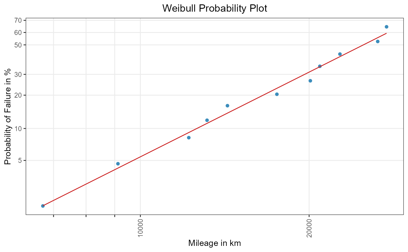
rr_weibull <- rank_regression(shock_cdf, distribution = "weibull")
rr_weibull
#> Rank Regression
#> Coefficients:
#>      mu    sigma
#> 10.2596   0.3632

# Probability plot:
weibull_grid <- plot_prob(
  shock_cdf,
  distribution = "weibull",
  title_main = "Weibull Probability Plot",
  title_x = "Mileage in km",
  title_y = "Probability of Failure in %",
  title_trace = "Defectives",
  plot_method = "ggplot2"
)

# Add regression line:
weibull_plot <- plot_mod(
  weibull_grid,
  x = rr_weibull,
  title_trace = "Rank Regression"
)

weibull_plot
Figure 1: RR for a two-parametric Weibull distribution.
ML for two-parameter Weibull distribution
# Again estimating Weibull:
ml_weibull <- ml_estimation(
  shock_tbl,
  distribution = "weibull"
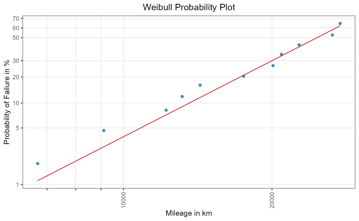
)

ml_weibull
#> Maximum Likelihood Estimation
#> Coefficients:
#>      mu    sigma
#> 10.2299   0.3164

# Add ML estimation to weibull_grid:
weibull_plot2 <- plot_mod(
  weibull_grid,
  x = ml_weibull,
  title_trace = "Maximum Likelihood"
)

weibull_plot2
Figure 2: ML for a two-parametric Weibull distribution.
ML for two- and three-parameter log-normal distribution
Finally, two- and three-parametric log-normal distributions are
fitted to the alloy data using maximum likelihood.
# Two-parameter log-normal:
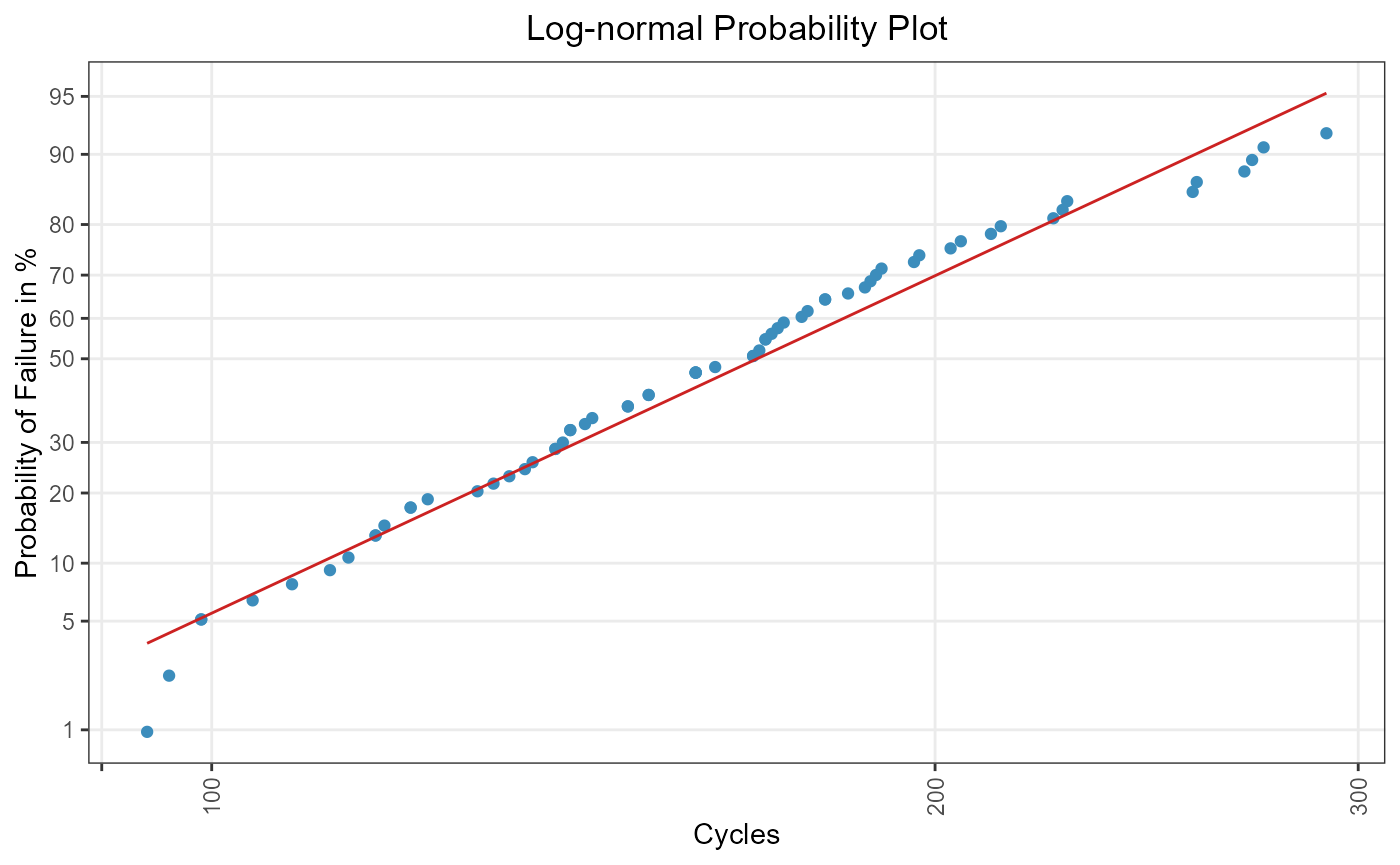
ml_lognormal <- ml_estimation(
  alloy_tbl,
  distribution = "lognormal"
)

ml_lognormal
#> Maximum Likelihood Estimation
#> Coefficients:
#>     mu   sigma
#> 5.1278  0.3276

# Three-parameter Log-normal:
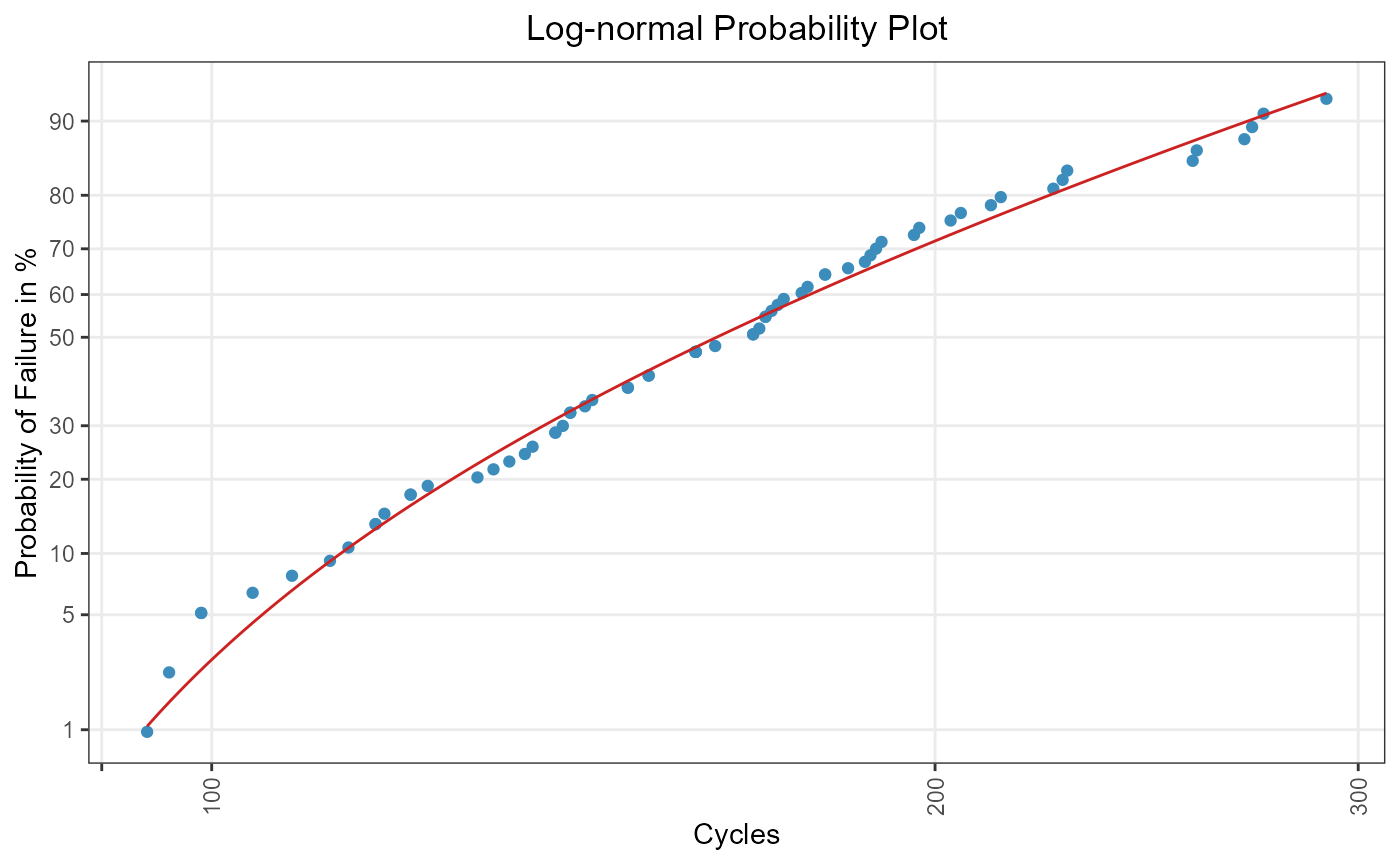
ml_lognormal3 <- ml_estimation(
  alloy_tbl,
  distribution = "lognormal3"
)

ml_lognormal3
#> Maximum Likelihood Estimation
#> Coefficients:
#>      mu    sigma    gamma
#>  4.5015   0.6132  72.0727
# Constructing probability plot:
tbl_cdf_john <- estimate_cdf(alloy_tbl, "johnson")

lognormal_grid <- plot_prob(
  tbl_cdf_john,
  distribution = "lognormal",
  title_main = "Log-normal Probability Plot",
  title_x = "Cycles",
  title_y = "Probability of Failure in %",
  title_trace = "Failed units",
  plot_method = "ggplot2"
)

# Add two-parametric model to grid:
lognormal_plot <- plot_mod(
  lognormal_grid,
  x = ml_lognormal,
  title_trace = "Two-parametric log-normal"
)

lognormal_plot
Figure 3: ML for a two-parametric log-normal distribution.
# Add three-parametric model to lognormal_plot:
lognormal3_plot <- plot_mod(
  lognormal_grid,
  x = ml_lognormal3,
  title_trace = "Three-parametric log-normal"
)

lognormal3_plot
Figure 4: ML for a three-parametric log-normal distribution.
Berkson, J.: Are There Two Regressions?, Journal of the American Statistical Association 45 (250), DOI: 10.2307/2280676, 1950, pp. 164-180↩︎
ReliaSoft Corporation: Life Data Analysis Reference Book, online: ReliaSoft, accessed 19 December 2020↩︎
Genschel, U.; Meeker, W. Q.: A Comparison of Maximum Likelihood and Median-Rank Regression for Weibull Estimation, in: Quality Engineering 22 (4), DOI: 10.1080/08982112.2010.503447, 2010, pp. 236-255↩︎
Meeker, W. Q.; Escobar, L. A.: Statistical Methods for Reliability Data, New York, Wiley series in probability and statistics, 1998, p. 630↩︎
Meeker, W. Q.; Escobar, L. A.: Statistical Methods for Reliability Data, New York, Wiley series in probability and statistics, 1998, p. 131↩︎