Life Data Analysis Part I - Estimation of Failure Probabilities
A Non-parametric Approach
Tim-Gunnar Hensel
David Barkemeyer
2022-03-30
Source:vignettes/Life_Data_Analysis_Part_I.Rmd
Life_Data_Analysis_Part_I.RmdThis document presents non-parametric estimation methods for the computation of failure probabilities of complete data (failures) taking (multiple) right-censored units into account. A unit can be either a single component, an assembly or an entire system.
Furthermore, the estimation results are presented in distribution-specific probability plots.
Introduction to Life Data Analysis
If the lifetime (or any other damage-equivalent quantity such as distance or load cycles) of a unit is considered to be a continuous random variable T, then the probability that a unit has failed at t is defined by its CDF (cumulative distribution function) F(t).
\[ P(T\leq t) = F(t) \]
In order to obtain an estimate of the CDF for each observation \(t_1, t_2, ..., t_n\) two approaches are possible. Using a parametric lifetime distribution requires that the underlying assumptions for the sample data are valid. If the distribution-specific assumptions are correct, the model parameters can be estimated and the CDF is computable. But if assumptions are not held, interpretations and derived conclusions are not reliable.
A more general approach for the calculation of cumulative failure probabilities is to use non-parametric statistical estimators \(\hat{F}(t_1), \hat{F}(t_2), ..., \hat{F}(t_n)\). In comparison to a parametric distribution no general assumptions must be held. For non-parametric estimators, an ordered sample of size \(n\) is needed. Starting at \(1\), the ranks \(i \in \{1, 2, ..., n \}\) are assigned to the ascending sorted sample values. Since there is a known relationship between ranks and corresponding ranking probabilities a CDF can be determined.
But rank distributions are systematically skewed distributions and thus the median value instead of the expected value \(E\left[F\left(t_i\right)\right] = \frac{i}{n + 1}\) is used for the estimation 1. This skewness is visualized in Figure 1.
library(dplyr) # data manipulation
library(ggplot2) # visualization

x <- seq(0, 1, length.out = 100) # CDF
n <- 10 # sample size
i <- c(1, 3, 5, 7, 9) # ranks
r <- n - i + 1 # inverse ranking

df_dens <- expand.grid(cdf = x, i = i) %>%
  mutate(n = n, r = n - i + 1, pdf = dbeta(x = x, shape1 = i, shape2 = r))

densplot <- ggplot(data = df_dens, aes(x = cdf, y = pdf, colour = as.factor(i))) +
  geom_line() +
  scale_colour_discrete(guide = guide_legend(title = "i")) +
  theme_bw() +
  labs(x = "Failure Probability", y = "Density")
densplot
Figure 1: Densities for different ranks i in samples of size n = 10.
Failure Probability Estimation
In practice, a simplification for the calculation of the median value, also called median rank, is made. The formula of Benard’s approximation is given by
\[\hat{F}(t_i) \approx \frac{i - 0,3}{n + 0,4} \]
and is described in The Plotting of Observations on Probability Paper 2.
However, this equation only provides valid estimates for failure
probabilities if all units in the sample are defectives
(estimate_cdf(methods = "mr", ...)).
In field data analysis, however, the sample mainly consists of intact units and only a small fraction of units failed. Units that have no damage at the point of analysis and also have not reached the operating time or mileage of units that have already failed, are potential candidates for future failures. As these, for example, still are likely to fail during a specific time span, like the guarantee period, the CDF must be adjusted upwards by these potential candidates.
A commonly used method for correcting probabilities of (multiple)
right-censored data is Johnson’s method
(estimate_cdf(methods = "johnson", ...)). By this method,
all units that are included in the period looked at are sorted in an
ascending order of their operating time (or any other damage-equivalent
quantity). If there are units that have not failed before the
i-th failure, an adjusted rank for the i-th failure is
formed. This correction takes the potential candidates into account and
increases the rank number. In consequence, a higher rank leads to a
higher failure probability. This can be seen in Figure 1.
The rank adjustment is determined with:
\[j_i = j_{i-1} + x_i \cdot I_i, \;\; with \;\; j_0 = 0\]
Here, \(j_ {i-1}\) is the adjusted rank of the previous failure, \(x_i\) is the number of defectives at \(t_i\) and \(I_i\) is the increment that corrects the considered rank by the potential candidates.
\[I_i=\frac{(n+1)-j_{i-1}}{1+(n-n_i)}\]
The sample size is \(n\) and \(n_i\) is the number of units that have a lower \(t\) than the i-th unit. Once the adjusted ranks are calculated, the CDF can be estimated according to Benard’s approximation.
Other methods in {weibulltools} that can also handle (multiple)
right-censored data are the Kaplan-Meier estimator
(estimate_cdf(methods = "kaplan", ...)) and the
Nelson-Aalen estimator
(estimate_cdf(methods = "nelson", ...)).
Probability Plotting
After computing failure probabilities a method called probability plotting is applicable. It is a graphical goodness of fit technique that is used in assessing whether an assumed distribution is appropriate to model the sample data.
The axes of a probability plot are transformed in such a way that the
CDF of a specified model is represented through a straight
line. If the plotted points (plot_prob()) lie on an
approximately straight line it can be said that the chosen distribution
is adequate.
The two-parameter Weibull distribution can be parameterized with parameters \(\mu\) and \(\sigma\) such that the CDF is characterized by the following equation:
\[F(t)=\Phi_{SEV}\left(\frac{\log(t) - \mu}{\sigma}\right)\]
The advantage of this representation is that the Weibull is part of the (log-)location-scale family. A linearized representation of this CDF is:
\[\Phi^{-1}_{SEV}\left[F(t)\right]=\frac{1}{\sigma} \cdot \log(t) - \frac{\mu}{\sigma}\]
This leads to the following transformations regarding the axes:
- Abscissa: \(x = \log(t)\)
- Ordinate: \(y = \Phi^{-1}_{SEV}\left[F(t)\right]\), which is the quantile function of the SEV (smallest extreme value) distribution and can be written out with \(\log\left\{-\log\left[1-F(t)\right]\right\}\).
Another version of the Weibull CDF with parameters \(\eta\) and \(\beta\) results in a CDF that is defined by the following equation:
\[F(t)=1-\exp\left[ -\left(\frac{t}{\eta}\right)^{\beta}\right]\]
Then a linearized version of the CDF is:
\[ \log\left\{-\log\left[1-F(t)\right]\right\} = \beta \cdot \log(t) - \beta \cdot \log(\eta)\]
Transformations regarding the axes are:
- Abscissa: \(x = \log(t)\)
- Ordinate: \(y = \log\left\{-\log\left[1-F(t)\right]\right\}\).
It can be easily seen that the parameters can be converted into each other. The corresponding equations are:
\[\beta = \frac{1}{\sigma}\]
and
\[\eta = \exp\left(\mu\right).\]
Data: Shock Absorber
To apply the introduced methods of non-parametric failure probability
estimation and probability plotting the shock data is used.
In this dataset kilometer-dependent problems that have occurred on shock
absorbers are reported. In addition to failed items the dataset also
contains non-defectives (censored) observations. The data can
be found in Statistical Methods for Reliability Data 3.
For consistent handling of the data, {weibulltools} introduces the
function reliability_data() that converts the original
dataset into a wt_reliability_data object. This formatted
object allows to easily apply the presented methods.
shock_tbl <- reliability_data(data = shock, x = distance, status = status)
shock_tbl
#> Reliability Data with characteristic x: 'distance':
#> # A tibble: 38 x 3
#>        x status id
#>    <int>  <dbl> <chr>
#>  1  6700      1 ID1
#>  2  6950      0 ID2
#>  3  7820      0 ID3
#>  4  8790      0 ID4
#>  5  9120      1 ID5
#>  6  9660      0 ID6
#>  7  9820      0 ID7
#>  8 11310      0 ID8
#>  9 11690      0 ID9
#> 10 11850      0 ID10
#> # ... with 28 more rows
Estimation of Failure Probabilities with {weibulltools}
First, we are interested in how censored observations influence the
estimation of failure probabilities in comparison to the case where only
failed units are considered. To deal with survived and failed units we
will use estimate_cdf() with
methods = "johnson", whereas methods = "mr"
only considers failures.
# Estimate CDF with both methods:
cdf_tbl <- estimate_cdf(shock_tbl, methods = c("mr", "johnson"))
#> The 'mr' method only considers failed units (status == 1) and does not retain intact units (status == 0).

# First case where only failed units are taken into account:
cdf_tbl_mr <- cdf_tbl %>% filter(cdf_estimation_method == "mr")
cdf_tbl_mr
#> CDF estimation for method 'mr':
#> # A tibble: 11 x 6
#>    id        x status  rank   prob cdf_estimation_method
#>    <chr> <int>  <dbl> <dbl>  <dbl> <chr>
#>  1 ID1    6700      1     1 0.0614 mr
#>  2 ID5    9120      1     2 0.149  mr
#>  3 ID13  12200      1     3 0.237  mr
#>  4 ID15  13150      1     4 0.325  mr
#>  5 ID19  14300      1     5 0.412  mr
#>  6 ID20  17520      1     6 0.5    mr
#>  7 ID27  20100      1     7 0.588  mr
#>  8 ID31  20900      1     8 0.675  mr
#>  9 ID32  22700      1     9 0.763  mr
#> 10 ID34  26510      1    10 0.851  mr
#> 11 ID36  27490      1    11 0.939  mr

# Second case where both, survived and failed units are considered:
cdf_tbl_john <- cdf_tbl %>% filter(cdf_estimation_method == "johnson")
cdf_tbl_john
#> CDF estimation for method 'johnson':
#> # A tibble: 38 x 6
#>    id        x status  rank    prob cdf_estimation_method
#>    <chr> <int>  <dbl> <dbl>   <dbl> <chr>
#>  1 ID1    6700      1  1     0.0182 johnson
#>  2 ID2    6950      0 NA    NA      johnson
#>  3 ID3    7820      0 NA    NA      johnson
#>  4 ID4    8790      0 NA    NA      johnson
#>  5 ID5    9120      1  2.09  0.0465 johnson
#>  6 ID6    9660      0 NA    NA      johnson
#>  7 ID7    9820      0 NA    NA      johnson
#>  8 ID8   11310      0 NA    NA      johnson
#>  9 ID9   11690      0 NA    NA      johnson
#> 10 ID10  11850      0 NA    NA      johnson
#> # ... with 28 more rows
If we compare both outputs we can see that survivors reduce the probabilities. But this is just that what was expected since undamaged units with longer or equal lifetime characteristic x let us gain confidence in the product.
Probability Plotting with {weibulltools}
The estimated probabilities should now be presented in a probability
plot. With plot_prob() probability plots for several
lifetime distributions can be constructed and estimates of multiple
methods can be displayed at once.
Weibull Probability Plot
# Weibull grid for estimated probabilities:
weibull_grid <- plot_prob(
  cdf_tbl,
  distribution = "weibull",
  title_main = "Weibull Probability Plot",
  title_x = "Mileage in km",
  title_y = "Probability of Failure in %",
  title_trace = "Method",
  plot_method = "ggplot2"
)

weibull_grid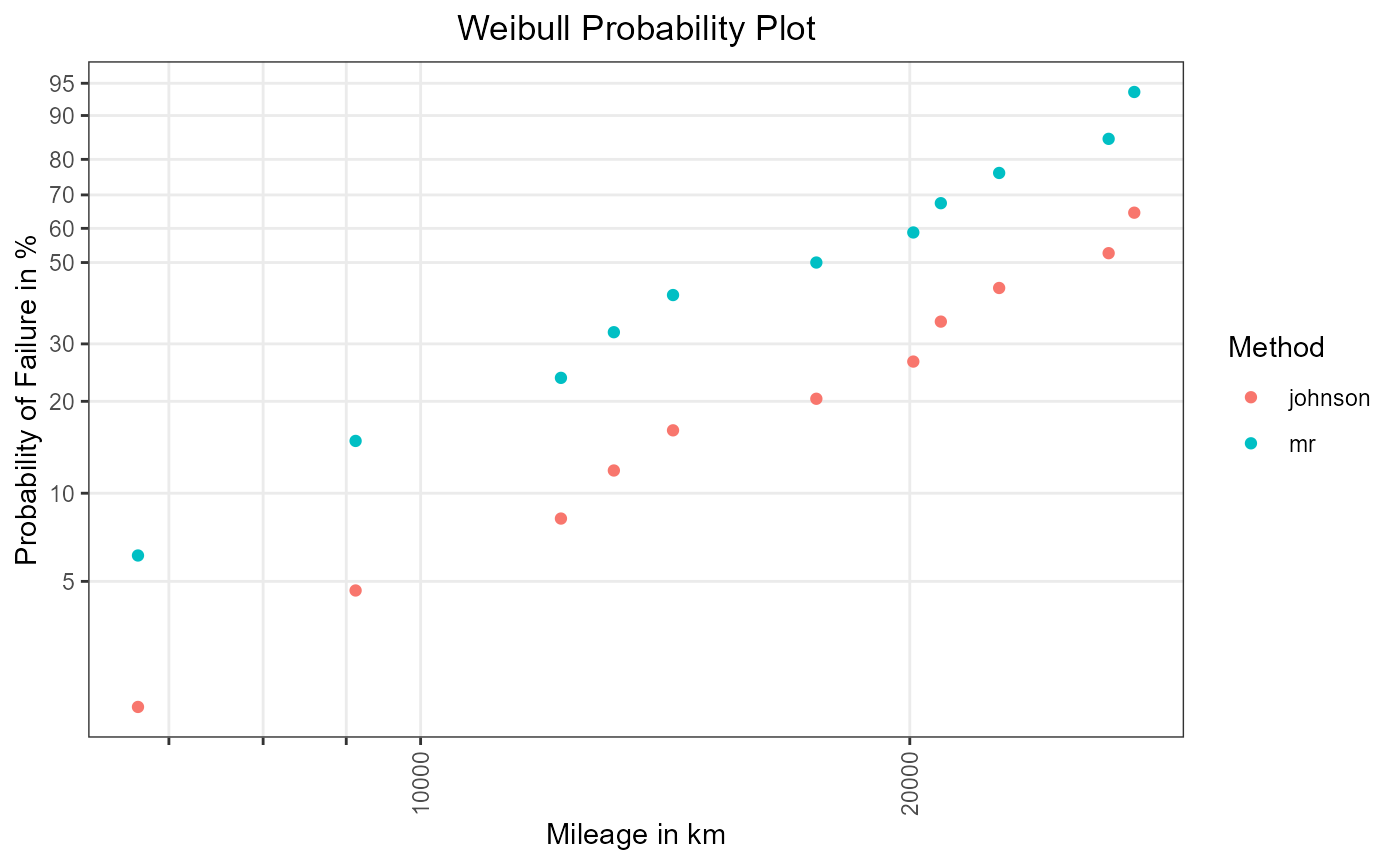
Figure 3: Plotting positions in Weibull grid.
Figure 3 shows that the consideration of survivors (orange points, Method: johnson) decreases the failure probability in comparison to the sole evaluation of failed items (green points, Method: mr).
Log-normal Probability Plot
Finally, we want to use a log-normal probability plot to visualize the estimated failure probabilities.
# Log-normal grid for estimated probabilities:
lognorm_grid <- plot_prob(
  cdf_tbl,
  distribution = "lognormal",
  title_main = "Log-normal Probability Plot",
  title_x = "Mileage in km",
  title_y = "Probability of Failure in %",
  title_trace = "Method",
  plot_method = "ggplot2"
)

lognorm_grid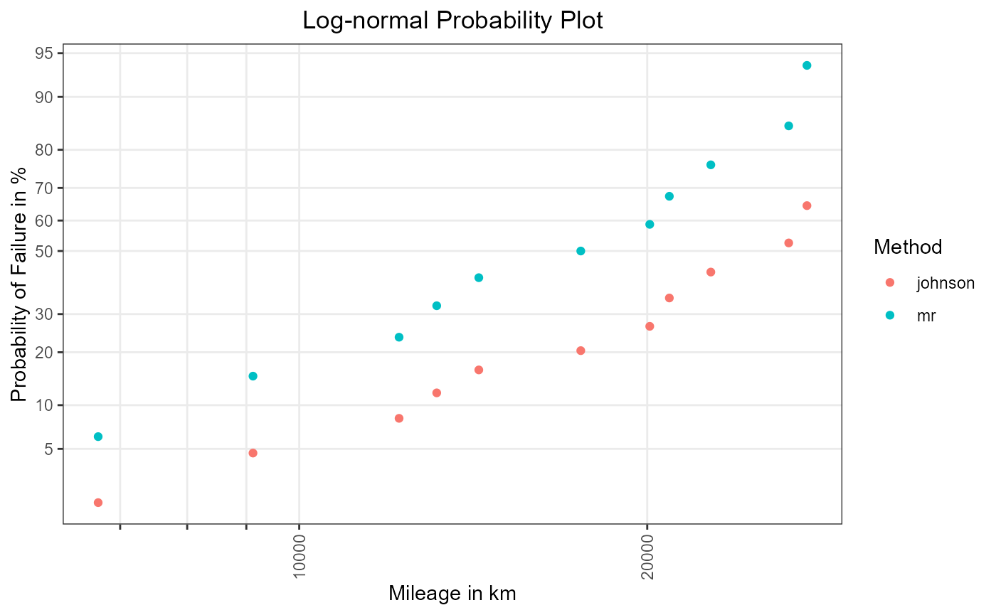
Figure 4: Plotting positions in log-normal grid.
On the basis of Figure 3 and Figure 4 we can
subjectively assess the goodness of fit of Weibull and log-normal. It
can be seen that in both grids, the plotted points roughly fall on a
straight line. Hence one can say that the Weibull as well as the
log-normal are good model candidates for the shock
data.
Kapur, K. C.; Lamberson, L. R.: Reliability in Engineering Design, New York: Wiley, 1977, pp. 297-301↩︎
Benard, A.; Bos-Levenbach, E. C.: The Plotting of Observations on Probability Paper, Statistica Neerlandica 7 (3), 1953, pp. 163-173↩︎
Meeker, W. Q.; Escobar, L. A.: Statistical Methods for Reliability Data, New York, Wiley series in probability and statistics, 1998, p. 630↩︎